Remember to download and put into data subdirectory:
Load the following into browser window:
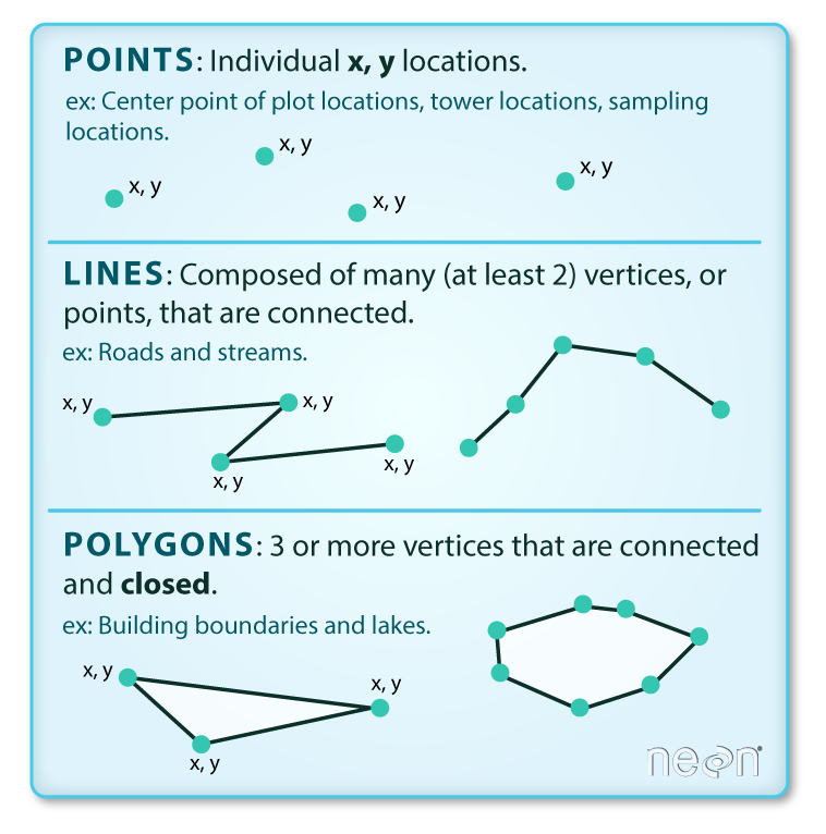
- [Vector Description]
Set-up R Console:
library(ggplot2)
Introduction to Vector Data
- Vector data includes points, lines, and polygons
- Examples include geopolitical boundaries, the location of field observations, and roads
- Vector data comes in a variety of formats
- shapefiles are are one of the most common
- They set of multiple files with the same name, but with different extensions
- We can see this by looking at the data in
data/HARV - This data includes data on some field plots at that Harvard Forest NEON site we’ve been working with
-
It is stored in the
plots_harvfiles and we can see there are four of them with different extensions - Work with vector data using the
sfpackage - We can read this data into R using
st_read - Let’s load in the plot data we just look at
library(sf)
plots_harv <- st_read("data/HARV/harv_plots.shp")
- When read read the data in we see information about it including
- The data has 5 features
- Each feature is one object, either a point, a line, or a polygon
- The geometry type is “POINT”, which means that the features are points
- The data has 2 fields
- Each field is a piece of information that is associated with each feature
- And there is information on the minimum and maximum spatial values in the dataset
- If we view this object we’ll see that it is a data frame with one row per vector object
- There are three columns
- The first two are the fields: id and plot_id, which in this case are both numerical plot IDs
- The last field is where the spatial information is stored and which is called
geometry - Since this is point data each object is stored as a pair of x and y coordinates
-
This makes it a special kind of data frame that can be used by spatial tools
- We can plot this data using a special geom,
geom_sf
ggplot() +
  geom_sf(data = plots_harv)
- We can also color vector data based on the values in the fields (or columns)
- For example, our plots have two different types, “Tower” and “Distributed”
- These are stored in the
plot_typefield - To color the points based on
plot_typewe add a mapping
ggplot() +
  geom_sf(data = plots_harv, mapping = aes(color = plot_type))
- Just like in scatter plots this mapping tells ggplot to “color the points based on `plot_type”
Combining multiple spatial layers
- We have the start This shows us the position of the plots, but it’s hard to learn much from this without some context
- So let’s load another vector object that shows the boundary of the research site
boundary_harv <- st_read("data/HARV/harv_boundary.shp")
- We can plot them together by adding two
geom_sflayers inggplot
ggplot() +
  geom_sf(data = boundary_harv) +
  geom_sf(data = plots_harv)
- The order of layers is important because they will plot on top of one another
- So if we’d plotted the plots first…
ggplot() +
  geom_sf(data = plots_harv) +
  geom_sf(data = boundary_harv)
- We wouldn’t have been able to see them.
- If we need to see through layers we can do this by setting the transparency using
alpha
ggplot() +
  geom_sf(data = plots_harv) +
  geom_sf(data = boundary_harv, alpha = 0.5)